Cumulative emissions

This example will walk through calculating and visulaizing cumulative emissions.

from itertools import cycle
import matplotlib.pyplot as plt
from matplotlib.ticker import AutoMinorLocator
from openclimate import Client
import numpy as np
import pandas as pd

We will first initialize a Client() object.

client = Client()

If you are using a jupyter enviornment, you will need to first client.jupyter. This patches the asyncio library to work in Jupyter envionrments using nest-asyncio.

client.jupyter

Get country codes

OpenClimate references each country by its two-letter ISO-3166 code. To access this in openclimate we can use the .parts() method to get all the “parts” of EARTH. Other codes we use are UN/LOCODEs for cities and LEI for companies. As a catch-all term, we call them an actor_id.

df_country = client.parts('EARTH')

Looking at the dataframe that’s returned, we have a column with each country’s actor_id.

df_country.head()

	actor_id	name	type	has_data	has_children	children_have_data
5	AD	Andorra	country	True	None	None
234	AE	United Arab Emirates	country	True	None	None
0	AF	Afghanistan	country	True	None	None
9	AG	Antigua and Barbuda	country	True	None	None
7	AI	Anguilla	country	True	None	None

Let’s save just the actor_id to a list

iso_and_name = list(zip(df_country['actor_id'], df_country['name']))

Which datasets are available?

To get a list of datasets available for an actor you can use the .emissions_datasets() method. Here I am asking for datasets with Candian emissions.

client.emissions_datasets('CA')

	actor_id	datasource_id	name	publisher	published	URL
0	CA	BP:statistical_review_june2022	Statistical Review of World Energy all data, 1...	BP	2022-06-01T00:00:00.000Z	https://www.bp.com/en/global/corporate/energy-...
1	CA	EDGARv7.0:ghg	Emissions Database for Global Atmospheric Rese...	JRC	2022-01-01T00:00:00.000Z	https://edgar.jrc.ec.europa.eu/dataset_ghg70
2	CA	GCB2022:national_fossil_emissions:v1.0	Data supplement to the Global Carbon Budget 20...	GCP	2022-11-04T00:00:00.000Z	https://www.icos-cp.eu/science-and-impact/glob...
3	CA	PRIMAP:10.5281/zenodo.7179775:v2.4	PRIMAP-hist_v2.4_no_extrap (scenario=HISTCR)	PRIMAP	2022-10-17T00:00:00.000Z	https://zenodo.org/record/7179775
4	CA	UNFCCC:GHG_ANNEX1:2019-11-08	UNFCCC GHG total without LULUCF, ANNEX I count...	UNFCCC	2019-11-08T00:00:00.000Z	https://di.unfccc.int/time_series
5	CA	climateTRACE:country_inventory	climate TRACE: country inventory	climate TRACE	2022-12-02T00:00:00.000Z	https://climatetrace.org/inventory
6	CA	WRI:climate_watch_historical_ghg:2022	Climate Watch Historical GHG Emissions	WRI	2022-01-01T00:00:00.000Z	https://www.climatewatchdata.org/ghg-emissions
7	CA	IEA:GHG_energy_highlights:2022	Greenhouse Gas Emissions from Energy Highlights	IEA	2022-09-01T00:00:00.000Z	https://www.iea.org/data-and-statistics/data-p...

You can return datasets for multiple actors at once by passing them as a callable, such as a list or tuple. Here I am asking for Canadian and Italian emission datasets, but only returning a sample of 5 records.

client.emissions_datasets(['CA', 'IT']).sample(5)

	actor_id	datasource_id	name	publisher	published	URL
7	CA	IEA:GHG_energy_highlights:2022	Greenhouse Gas Emissions from Energy Highlights	IEA	2022-09-01T00:00:00.000Z	https://www.iea.org/data-and-statistics/data-p...
4	CA	UNFCCC:GHG_ANNEX1:2019-11-08	UNFCCC GHG total without LULUCF, ANNEX I count...	UNFCCC	2019-11-08T00:00:00.000Z	https://di.unfccc.int/time_series
10	IT	GCB2022:national_fossil_emissions:v1.0	Data supplement to the Global Carbon Budget 20...	GCP	2022-11-04T00:00:00.000Z	https://www.icos-cp.eu/science-and-impact/glob...
16	IT	openGHGmap:R2021A	European OpenGHGMap	NTNU	2021-01-01T00:00:00.000Z	https://openghgmap.net/data/
14	IT	climateTRACE:country_inventory	climate TRACE: country inventory	climate TRACE	2022-12-02T00:00:00.000Z	https://climatetrace.org/inventory

Get emissions

If we just pass an actor_id to the .emissions() method, all the emissions will be returned.

df_tmp = client.emissions(actor_id='US')
df_tmp.head()

	actor_id	year	total_emissions	datasource_id
0	US	1990	5275397531	BP:statistical_review_june2022
1	US	1991	5225911642	BP:statistical_review_june2022
2	US	1992	5308410257	BP:statistical_review_june2022
3	US	1993	5412149078	BP:statistical_review_june2022
4	US	1994	5505379237	BP:statistical_review_june2022

Keep in mind that this will return all the data for that actor. Below are the datasets available.

set(df_tmp['datasource_id'])

{'BP:statistical_review_june2022',
 'EDGARv7.0:ghg',
 'GCB2022:national_fossil_emissions:v1.0',
 'IEA:GHG_energy_highlights:2022',
 'PRIMAP:10.5281/zenodo.7179775:v2.4',
 'UNFCCC:GHG_ANNEX1:2019-11-08',
 'WRI:climate_watch_historical_ghg:2022',
 'carbon_monitor:2022_12_14',
 'climateTRACE:country_inventory'}

In most cases, we want to filter this and use a particular dataset. We can do that with the datasource_id parameter.

df_tmp = client.emissions(actor_id='US', datasource_id='PRIMAP:10.5281/zenodo.7179775:v2.4')

As a sanity check, let’s look at which datasets are returned

set(df_tmp['datasource_id'])

{'PRIMAP:10.5281/zenodo.7179775:v2.4'}

As you see, only PRIMAP was returned.

Get emissions for all countries

Now let’s get emissions for all countries

%%time
iso_codes = [iso_code[0] for iso_code in iso_and_name]
df_emissions = client.emissions(
    actor_id=iso_codes,
    datasource_id='PRIMAP:10.5281/zenodo.7179775:v2.4'
)

CPU times: user 5.52 s, sys: 289 ms, total: 5.81 s
Wall time: 20.3 s

This takes about 30 seconds to retrieve all that data, even with asyncio working behind the scenes. This outputs a massive dataframe with the data from all countries concatenated together

df_emissions.sample(5)

	actor_id	year	total_emissions	datasource_id
492	BG	2015	62400000	PRIMAP:10.5281/zenodo.7179775:v2.4
215	GT	1832	549000	PRIMAP:10.5281/zenodo.7179775:v2.4
117	GN	1751	1050000	PRIMAP:10.5281/zenodo.7179775:v2.4
240	PW	1908	20300	PRIMAP:10.5281/zenodo.7179775:v2.4
384	IL	1907	406000	PRIMAP:10.5281/zenodo.7179775:v2.4

Calculate cumulative emissions

let’s first make sure all the datasets have the same starting year

all([df_emissions.loc[df_emissions['actor_id']==iso_code, 'year'].min() for iso_code in set(df_emissions['actor_id'])])

True

Now we can calculate cumulative emissions

df_out = df_emissions.assign(cumulative_emissions = df_emissions.groupby('actor_id')['total_emissions'].cumsum())

Now we have a column for cumulative emissions

df_out.head()

	actor_id	year	total_emissions	datasource_id	cumulative_emissions
32	AD	1750	3740	PRIMAP:10.5281/zenodo.7179775:v2.4	3740
33	AD	1751	3750	PRIMAP:10.5281/zenodo.7179775:v2.4	7490
34	AD	1752	3760	PRIMAP:10.5281/zenodo.7179775:v2.4	11250
35	AD	1753	3770	PRIMAP:10.5281/zenodo.7179775:v2.4	15020
36	AD	1754	3780	PRIMAP:10.5281/zenodo.7179775:v2.4	18800

Rank country by cumulative emissions

Now that we now the cumulative emission, we can rank the countries by the cumulative emissions in the most recent year.

last_year = df_out['year'].max()
df_sorted = (
    df_out.loc[df_out['year'] == last_year, ['actor_id', 'cumulative_emissions', 'year']]
    .sort_values(by='cumulative_emissions', ascending=False)
)

df_sorted['rank'] = df_sorted['cumulative_emissions'].rank(ascending=False)

Here are the top 10 cumulative emitters

pd.merge(df_sorted.loc[df_sorted['rank'] <= 10], df_country[['actor_id', 'name']], on='actor_id')

	actor_id	cumulative_emissions	year	rank	name
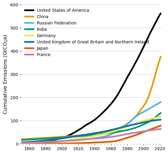
0	US	561240060000	2021	1.0	United States of America
1	CN	375048000000	2021	2.0	China
2	RU	179731600000	2021	3.0	Russian Federation
3	IN	132717000000	2021	4.0	India
4	DE	117760000000	2021	5.0	Germany
5	GB	104375500000	2021	6.0	United Kingdom of Great Britain and Northern I...
6	JP	78204570000	2021	7.0	Japan
7	FR	64192400000	2021	8.0	France
8	UA	52563900000	2021	9.0	Ukraine
9	BR	47231630000	2021	10.0	Brazil

The United States and China are the top two emitters, with the U.S. emitting about 50% more emissions than China over the period from 1750 to 2021.

561240060000 / 375048000000

1.4964486145773341

Plot cumulative emissions

Now that we know the top emitters, we can plot a time series

fig = plt.figure(figsize=(6, 6))
ax = fig.add_subplot(111)

# top 8 emitters
top_emitters = list(df_sorted.head(8).actor_id)

# wong color palette (https://davidmathlogic.com/colorblind/#%23D81B60-%231E88E5-%23FFC107-%23004D40)
colors = ['#000000', '#E69F00', '#56B4E9', '#009E73', '#F0E442', '#0072B2', '#D55E00', '#CC79A7']

for actor_id, color in zip(top_emitters, cycle(colors)):
    actor_name = df_country.loc[df_country['actor_id'] == actor_id, 'name'].values[0]
    filt = df_out['actor_id'] == actor_id
    df_tmp = df_out.loc[filt]

    ax.plot(np.array(df_tmp['year']), np.array(df_tmp['cumulative_emissions']) / 10**9,
            linewidth=4,
            label = actor_name,
            color=color)

    ylim = [0, 600]
    ax.set_ylim(ylim)
    ax.set_xlim([1850, 2022])

    # Turn off the display of all ticks.
    ax.tick_params(which='both',     # Options for both major and minor ticks
                   top='off',        # turn off top ticks
                   left='off',       # turn off left ticks
                   right='off',      # turn off right ticks
                   bottom='off')     # turn off bottom ticks

    # Remove x tick marks
    plt.setp(ax.get_xticklabels(), rotation=0)

    # Hide the right and top spines
    ax.spines['right'].set_visible(False)
    ax.spines['left'].set_visible(False)
    ax.spines['top'].set_visible(False)
    ax.spines['bottom'].set_visible(False)

    # Only show ticks on the left and bottom spines
    ax.yaxis.set_ticks_position('left')
    ax.xaxis.set_ticks_position('bottom')

    # major/minor tick lines
    ax.xaxis.set_minor_locator(AutoMinorLocator(5))
    ax.grid(axis='y',
            which='major',
            color=[0.8, 0.8, 0.8], linestyle='-')

    ax.set_ylabel("Cumulative Emissions (GtCO$_2$e)", fontsize=12)
    ax.legend(loc='upper left', frameon=False)