Canada Emissions Breakdown

In this notebook we will explore a territorial breakdown of Canadian emissions into provinces using data submitted to UNFCCC.

from itertools import cycle
import matplotlib.pyplot as plt
from matplotlib.ticker import AutoMinorLocator
import pandas as pd

Matplotlib is building the font cache; this may take a moment.

from openclimate import Client
client = Client()
client.jupyter

Let’s display all of dataset’s available for Canada

client.emissions_datasets('CA')

	actor_id	datasource_id	name	publisher	published	URL
0	CA	BP:statistical_review_june2022	Statistical Review of World Energy all data, 1...	BP	2022-06-01T00:00:00.000Z	https://www.bp.com/en/global/corporate/energy-...
1	CA	EDGARv7.0:ghg	Emissions Database for Global Atmospheric Rese...	JRC	2022-01-01T00:00:00.000Z	https://edgar.jrc.ec.europa.eu/dataset_ghg70
2	CA	GCB2022:national_fossil_emissions:v1.0	Data supplement to the Global Carbon Budget 20...	GCP	2022-11-04T00:00:00.000Z	https://www.icos-cp.eu/science-and-impact/glob...
3	CA	PRIMAP:10.5281/zenodo.7179775:v2.4	PRIMAP-hist_v2.4_no_extrap (scenario=HISTCR)	PRIMAP	2022-10-17T00:00:00.000Z	https://zenodo.org/record/7179775
4	CA	UNFCCC:GHG_ANNEX1:2019-11-08	UNFCCC GHG total without LULUCF, ANNEX I count...	UNFCCC	2019-11-08T00:00:00.000Z	https://di.unfccc.int/time_series
5	CA	climateTRACE:country_inventory	climate TRACE: country inventory	climate TRACE	2022-12-02T00:00:00.000Z	https://climatetrace.org/inventory
6	CA	WRI:climate_watch_historical_ghg:2022	Climate Watch Historical GHG Emissions	WRI	2022-01-01T00:00:00.000Z	https://www.climatewatchdata.org/ghg-emissions
7	CA	IEA:GHG_energy_highlights:2022	Greenhouse Gas Emissions from Energy Highlights	IEA	2022-09-01T00:00:00.000Z	https://www.iea.org/data-and-statistics/data-p...

Now let’s gather emissions data for Canada from UNFCCC as well as emissions for each province from ECCC. Finally, let’s gather population data for Canada and its provinces from 2017 (this is the most recent year we have emissions for all provinces).

# canadian emissions
df_ca = client.emissions('CA', 'UNFCCC:GHG_ANNEX1:2019-11-08')

# canadian province names
df_parts = client.parts('CA', part_type='adm1')[['actor_id', 'name']]

# province emissions
df_prov = client.emissions(df_parts.actor_id, 'ECCC:GHG_inventory:2022-04-13')

# candian population in 2017
df_ca_pop = (
    client.population('CA')
    .loc[lambda x: x['year'] == 2017, ['actor_id', 'year', 'population']]
)

# province population in 2017
df_prov_pop = (
    client.population(df_parts.actor_id)
    .loc[lambda x: x['year'] == 2017, ['actor_id', 'year', 'population']]
)

Now let’s select Canadian emissions and provincial emissions for 2020. I know it’s not the same year as population, but let’s assum popluation hasn’t changed signifcantly in three years. We are also going to convert to megatonnes of CO2 equivalents by dividing by dividing the emissions by a million.

# national emissions in MTCO2e
national = df_ca.loc[df_ca['year'] == 2020, 'total_emissions'].values / 10**6

# province emissions and cumulative emissions in MTCO2e
df_out = (
    df_prov
    .loc[df_prov['year'] == 2020, ['total_emissions', 'actor_id']]
    .assign(total_emissions= lambda x: x['total_emissions'].div(10**6), inplace=True)
    .assign(percent_of_national = lambda x: (x['total_emissions'] / national) * 100)
    .sort_values(by='percent_of_national', ascending=False)
    .assign(cumulative = lambda x: x['percent_of_national'].cumsum())
    .merge(df_parts, on='actor_id')
    .merge(df_prov_pop, on='actor_id')
    .assign(percent_of_population = lambda x: (x['population'] / x['population'].sum()) * 100)
    .rename(columns={'total_emissions': 'total_emissions_[MTCO2e]'})
    .loc[:, ['actor_id', 'name', 'total_emissions_[MTCO2e]', 'percent_of_national',  'cumulative', 'population', 'percent_of_population']]
)

Now let’s display a table showing the province, emissions breakdown, and population.

df_out

	actor_id	name	total_emissions_[MTCO2e]	percent_of_national	cumulative	population	percent_of_population
0	CA-AB	Alberta	256.459542	38.143528	38.143528	4306039	11.674212
1	CA-ON	Ontario	149.584918	22.247940	60.391467	14279196	38.712694
2	CA-QC	Quebec	76.241175	11.339439	71.730907	8425996	22.843933
3	CA-SK	Saskatchewan	65.894159	9.800515	81.531422	1168057	3.166749
4	CA-BC	British Columbia	61.746788	9.183672	90.715094	4841078	13.124770
5	CA-MB	Manitoba	21.674064	3.223609	93.938703	1343371	3.642047
6	CA-NS	Nova Scotia	14.596446	2.170946	96.109649	957600	2.596174
7	CA-NB	New Brunswick	12.440907	1.850351	97.960000	760868	2.062809
8	CA-NL	Newfoundland and Labrador	9.500844	1.413072	99.373072	528430	1.432640
9	CA-PE	Prince Edward Island	1.609972	0.239453	99.612525	152784	0.414217
10	CA-NT	Northwest Territories	1.401465	0.208442	99.820966	44718	0.121236
11	CA-NU	Nunavut	0.602920	0.089673	99.910639	38243	0.103682
12	CA-YT	Yukon	0.600610	0.089329	99.999969	38669	0.104837

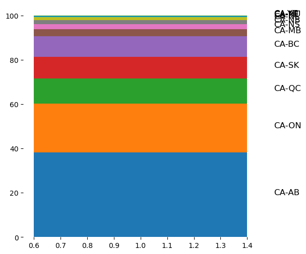
This shows that 5 provines (Albera, Ontario, Quebec, Saskatchewan, and British Columbia) make up over 90% of Canada’s overall emissions in 2020. Alberta, while only accounting for about 12% of Canada’s population contributes to 38% of the nation’s emissions. This is largely driven by oil/gas and agriculture sectors.

Finally, let’s make a first attempt at visulaizating this breakdow. This bar graph is clunky and could be improved.

fig = plt.figure(figsize=(6, 6))
ax = fig.add_subplot(111)

previous = 0
for iterator, row in df_out.iterrows():
    emissions = row['percent_of_national']
    cumulative = row['cumulative']
    actor_id = row['actor_id']
    ax.bar(1, emissions, bottom=previous, label=actor_id)
    previous = cumulative
    ax.text(1.5, previous - (emissions/2),
          actor_id,
          fontsize=12,
          color='k')

# Turn off the display of all ticks.
ax.tick_params(which='both',     # Options for both major and minor ticks
               top='off',        # turn off top ticks
               left='off',       # turn off left ticks
               right='off',      # turn off right ticks
               bottom='off')     # turn off bottom ticks

# Remove x tick marks
plt.setp(ax.get_xticklabels(), rotation=0)

# Hide the right and top spines
ax.spines['right'].set_visible(False)
ax.spines['left'].set_visible(False)
ax.spines['top'].set_visible(False)
ax.spines['bottom'].set_visible(False)

# Only show ticks on the left and bottom spines
ax.yaxis.set_ticks_position('left')
ax.xaxis.set_ticks_position('bottom')

# grid and tick marks
ax.set_yticks(np.arange(10, 110, 10))
ax.grid(axis='y',
        which='major',
        color=[0.8, 0.8, 0.8], linestyle='-')

ax.set_axisbelow(True)
ax.set_xticks([])
ax.set_title("Territorial Breakdown of Canada's 2020 emissions")
ax.set_ylabel("% of national emissions")

---------------------------------------------------------------------------
NameError                                 Traceback (most recent call last)
Cell In[7], line 37
     34 ax.xaxis.set_ticks_position('bottom')
     36 # grid and tick marks
---> 37 ax.set_yticks(np.arange(10, 110, 10))
     38 ax.grid(axis='y',
     39         which='major',
     40         color=[0.8, 0.8, 0.8], linestyle='-')
     42 ax.set_axisbelow(True)

NameError: name 'np' is not defined